
Working in notebooks
Orcapod's streams, sources, job nodes, run summaries, jobs and pipelines display themselves
when they are the last line of a notebook cell. This page is where a notebook user starts:
what each display shows, how to see more, and which page states each rule in full. The
pictures come from JupyterLab. Outside a notebook, print(stream.head()), print(summary) and
print(job.diagram()) give the same displays as text (print(stream) or print(job) does
not), and the samples below show that text.
The samples use the job from Part 5 of the tutorial, not run
yet, over the tutorial's dataset: to run them, first put workshop_data.py in your notebook's
working directory, as Get the dataset in Part 0
shows.
from workshop_data import make_datasetfrom orcapod import PipelineJob, function_podfrom orcapod.databases import InMemoryArrowDatabasefrom orcapod.sources import CSVSource
data_dir = make_dataset()
sessions = CSVSource(    str(data_dir / "sessions.csv"),    tag_columns=["subject_id", "session"], tag_only_columns=True,    source_id="sessions",)units = CSVSource(    str(data_dir / "units.csv"),    tag_columns=["subject_id", "session", "probe", "unit"], tag_only_columns=True,    source_id="units",)

@function_pod(output_keys="rate_hz")def firing_rate(n_spikes: int, duration_s: float) -> float:    return n_spikes / duration_s

@function_pod(output_keys="mean_rate_hz")def mean_rate(rate_hz: list[float]) -> float:    return sum(rate_hz) / len(rate_hz)

job = PipelineJob(name="workshop", database=InMemoryArrowDatabase())with job:    rates = firing_rate.pod(        units.select_data_columns(["n_spikes"]),        sessions.select_data_columns(["duration_s"]),        label="rates",    )    mean_rate.pod(        rates.group_by(["subject_id", "session"]).select_data_columns(["rate_hz"]),        label="session_means",    )
A stream at the end of a cell
Section titled “A stream at the end of a cell”In a notebook, a stream, source or job node shown at the end of a cell renders a short
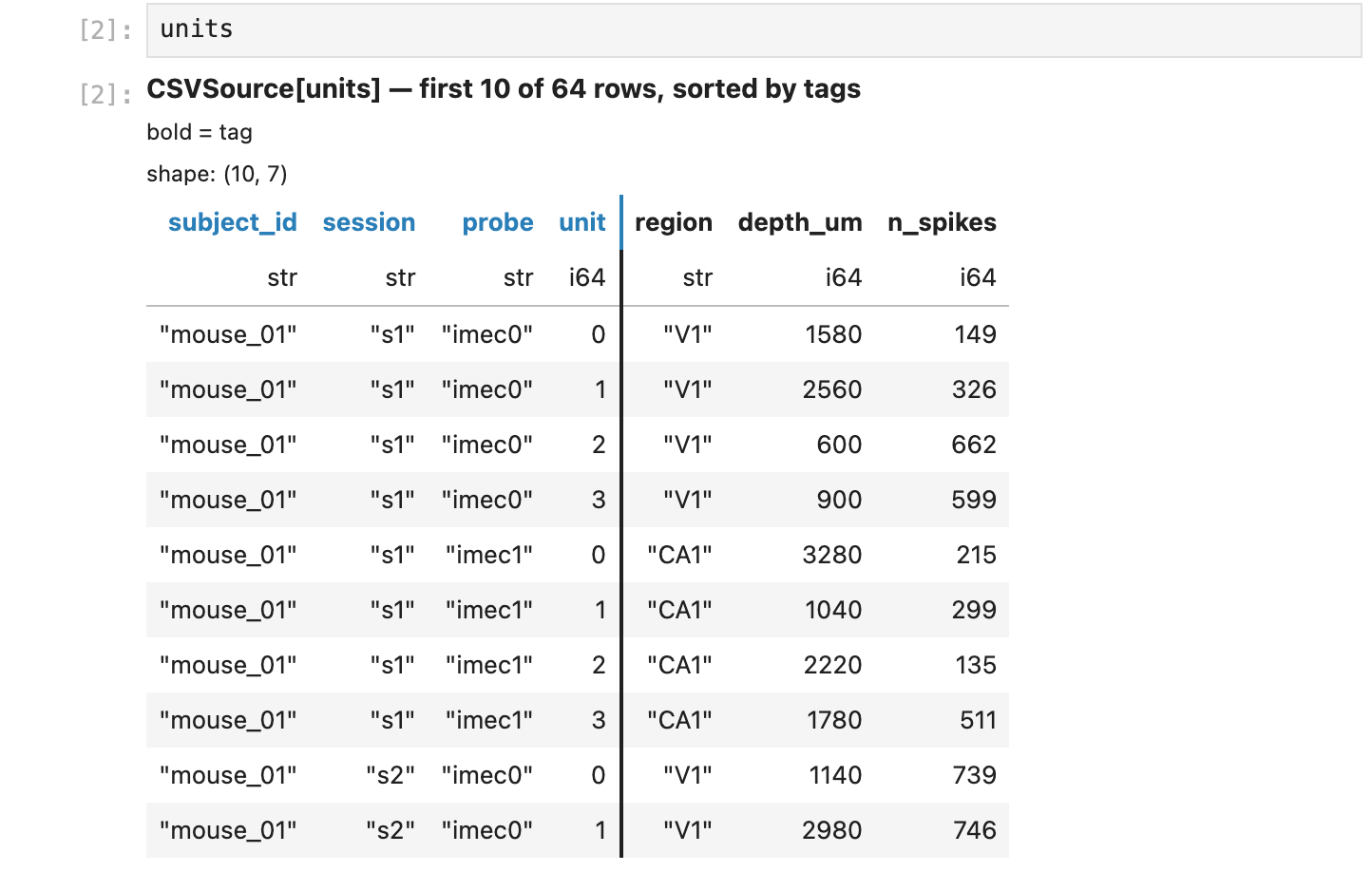
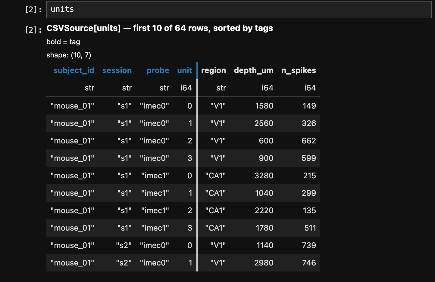
table: its first rows in tag order, with a line saying what they are. Here is units as the
last line of a cell:
What it shows (Looking at data states each rule in full):
- The header line names the object (its kind and its name) and says which rows are shown:
here
first 10 of 64 rows, sorted by tags. A source that reads only part of its table says so, as a SpiralDB source does ("10 rows read, sorted by tags, of about 63,349"). - Tag columns come first and are marked: in a notebook their headers are bold (in an accent colour), a vertical rule separates them from the data columns and a line under the header says "bold = tag". A data-tag is one column: the notebook preview shows it once, among the tags, marked as a tag.
- Large cells are summarised (an array as
ndarray float64 (2, 3), bytes asbytes (300 B), long text and long lists shortened);head().tablekeeps the full values.
The preview is head() asked for sort_by_tags, and neither ever computes anything: they
show only what is readily available, never compute, poll or deliver a row (they read only
what is held or stored, or make a bounded table read), never call your code (a function, a
predicate, a side effect) and never write to a database. So a job node shown before the job
has run has no rows: its header says not run, and the table shows its columns only.
In a terminal, print(stream.head()) prints the same preview as text. There, each tag
column's name starts with * ("* = tag"):
print(units.head(3))# CSVSource[units] — first 3 of 64 rows# * = tag# shape: (3, 7)# ┌─────────────┬──────────┬────────┬───────┬────────┬──────────┬──────────┐# │ *subject_id ┆ *session ┆ *probe ┆ *unit ┆ region ┆ depth_um ┆ n_spikes │# │ --- ┆ --- ┆ --- ┆ --- ┆ --- ┆ --- ┆ --- │# │ str ┆ str ┆ str ┆ i64 ┆ str ┆ i64 ┆ i64 │# ╞═════════════╪══════════╪════════╪═══════╪════════╪══════════╪══════════╡# │ mouse_01 ┆ s1 ┆ imec0 ┆ 0 ┆ V1 ┆ 1580 ┆ 149 │# │ mouse_01 ┆ s1 ┆ imec0 ┆ 1 ┆ V1 ┆ 2560 ┆ 326 │# │ mouse_01 ┆ s1 ┆ imec0 ┆ 2 ┆ V1 ┆ 600 ┆ 662 │# └─────────────┴──────────┴────────┴───────┴────────┴──────────┴──────────┘print(job.nodes["rates"].head())# FunctionJobNode[rates] — not run; run() fills it; node.as_source() shows every stored result# * = tag# shape: (0, 5)# ┌─────────────┬──────────┬────────┬───────┬─────────┐# │ *subject_id ┆ *session ┆ *probe ┆ *unit ┆ rate_hz │# │ --- ┆ --- ┆ --- ┆ --- ┆ --- │# │ str ┆ str ┆ str ┆ i64 ┆ f64 │# ╞═════════════╪══════════╪════════╪═══════╪═════════╡# └─────────────┴──────────┴────────┴───────┴─────────┘(head() does not sort, so its header does not say sorted by tags; the preview asks for
the sorted head.) What each kind of object shows before and after it is computed (a source,
a computed stream, a job node, a side-effect node) is the table "What each kind of object
shows" in Streams.
The run summary
Section titled “The run summary”job.run() (and await job.run_async()) returns a RunSummary: for each function node, how
many rows were computed, how many were read from the database, and how many failed. At the end
of a notebook cell it is shown as a table; print shows the same as text:
summary = job.run()print(summary)# Run of job 'workshop': all rows succeeded.# rates: 64 rows: 63 computed, 1 from store, 0 failed# session_means: 8 rows: 8 computed, 0 from store, 0 failed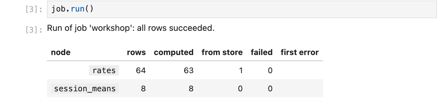
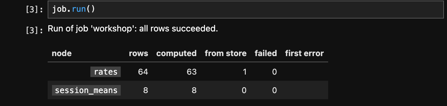
One row per function node: rows is every input row the run accounted for in the node
(computed, from store and failed, and for a node the run held, its held rows), computed
how many its function computed in this run, from store how many it read back from the
database instead, failed how many raised, and first error the first of those errors, with the call that
prints its full traceback (job.last_run.print_traceback("rates")). Here one rates row
was found in the store during the run itself (Part 5
of the tutorial explains why). A load-only run (job.run(load_only=True)) shows how many
rows each node loaded and how many had no stored result instead. The job keeps the summary as
job.last_run. A cell that ends with job.run(); (a semicolon) shows nothing. What a run
does when a function raises for a row is
Reading the run summary.
Seeing more rows
Section titled “Seeing more rows”After the run, every node holds the rows of that run, and its preview shows them. To see other rows:
node.head(n)shows the firstnrows;head(n, columns={"sort_by_tags": True})gives the rows the preview shows.node.run()at the end of a cell computes what is not computed yet and shows every row: in a notebook,stream.run()at the end of a cell computes and displays. A view of more than ten rows that nobody cut shows its first and last five rows, and its header gives the count.- The view that
head()orrun()returns cuts and orders its own rows, without reading or computing anything:view.head(n),view.tail(n),view.sort_by_tags(), and chains of them such asview.head(20).tail(10). - For every row, as a data frame or a table, use
as_polars_df(),as_pandas_df()oras_table(). A data frame at the end of a cell is shown by its own library.
means = job.nodes["session_means"]view = means.run() # the node holds a current run: this computes nothingprint(view.header())# FunctionJobNode[session_means] — all 8 rowsprint(view.tail(3))# FunctionJobNode[session_means] — last 3 of 8 rows# * = tag# shape: (3, 3)# ┌─────────────┬──────────┬──────────────┐# │ *subject_id ┆ *session ┆ mean_rate_hz │# │ --- ┆ --- ┆ --- │# │ str ┆ str ┆ f64 │# ╞═════════════╪══════════╪══════════════╡# │ mouse_03 ┆ s2 ┆ 5.059375 │# │ mouse_04 ┆ s1 ┆ 5.136458 │# │ mouse_04 ┆ s2 ┆ 5.129167 │# └─────────────┴──────────┴──────────────┘print(job.nodes["rates"].run().header())# FunctionJobNode[rates] — all 64 rowsA view holds the default columns only (tags and data). For system tags, source info and
the other hidden columns, ask the node: as_table(columns=...), as in
Part 8 of the tutorial. run() on each kind of
object is the table "What run() does on each kind of object" in
Streams.
The pipeline diagram
Section titled “The pipeline diagram”import warnings
from orcapod.errors import InDevelopmentWarning
warnings.filterwarnings("ignore", category=InDevelopmentWarning)In a notebook, a job or a pipeline shown at the end of a cell draws itself: a diagram of its
nodes (sources, operators, function pods, side-effect pods) and the streams between them,
laid out left to right. Here is job as the last line of a cell, after its run, with the
rates node selected:
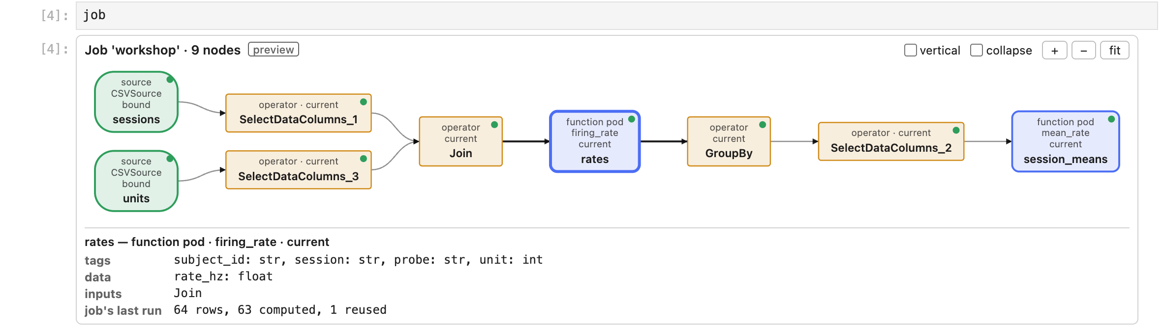
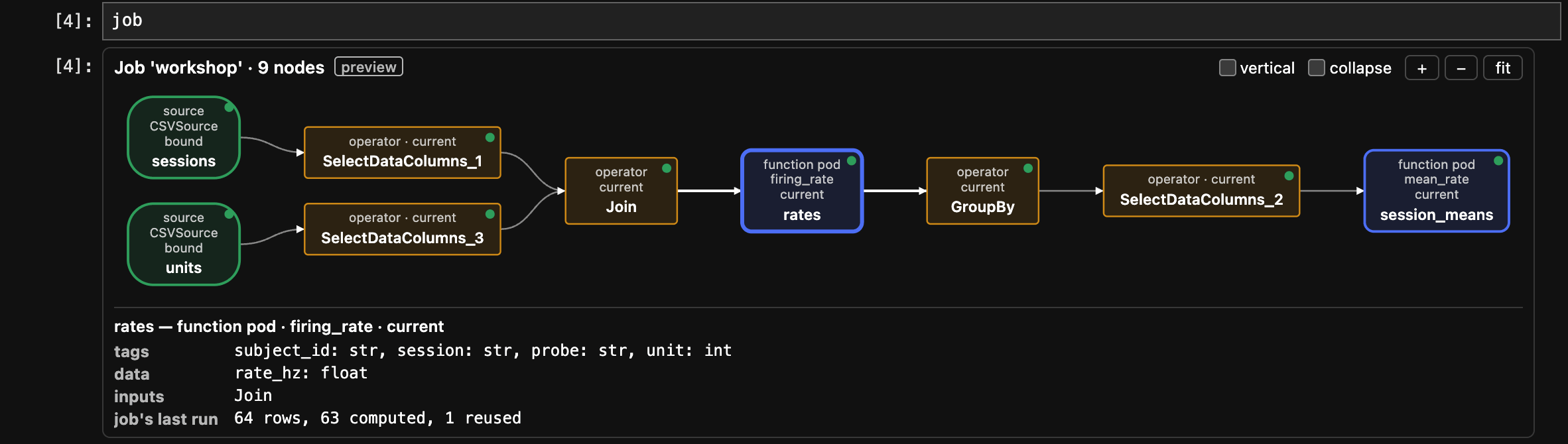
Seeing the graph states each of these in full:
- Moving and zooming. Drag to move it and use the
+,−andfitbuttons (or Ctrl or Cmd with the mouse wheel) to zoom; from the keyboard, focus the diagram and use the arrow keys to move it,+and-to zoom and0to fit, and Tab to reach the nodes. - A node's details. Click a node (or focus it and press Enter) to see its schema: its tag and data columns, the nodes it reads from and, for a job, its run status and the row counts of the job's last run.
- Statuses. Each node of a job shows one:
not run,current,stale,failed,loaded only,partial, orboundorunboundfor a source slot. Beforejob.run()every node but the sources saysnot run. - The
verticalandcollapsecheckboxes.direction="TB"lays the graph out top to bottom, andcollapse=Truefolds the steps that only choose, rename or join columns into the edge they lie on. In a notebook that runs scripts, theverticalandcollapsecheckboxes next to the zoom buttons switch between these layouts in place (collapseappears only when there is something to fold; neither appears above 100 nodes). - Nothing is computed. Drawing a diagram never computes anything.
- Saved with the notebook. The picture is part of the cell's output, so it stays in a
saved notebook and in an HTML export.
job.diagram().save("pipeline.html")writes it as a page that opens in any browser.
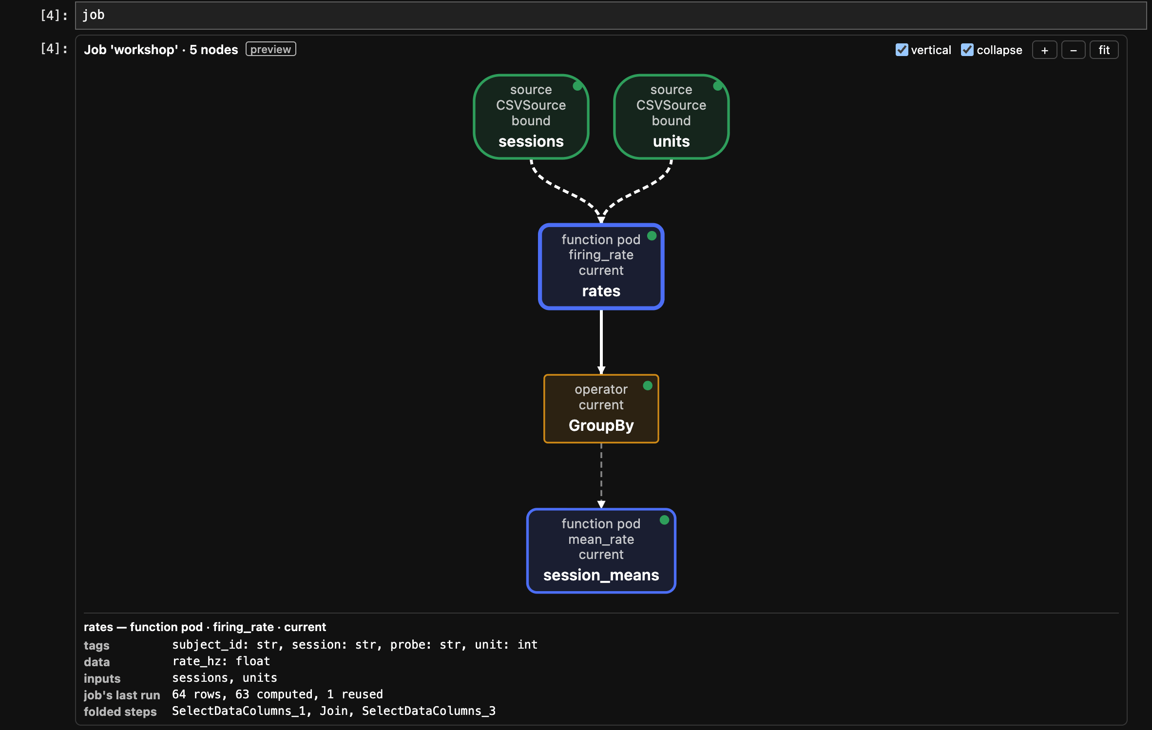
Here is the same diagram after ticking vertical and then collapse: five nodes, top to
bottom, with the column selections and the join folded into the dashed edges. rates stays
selected, and its details now list the steps folded into its inputs:
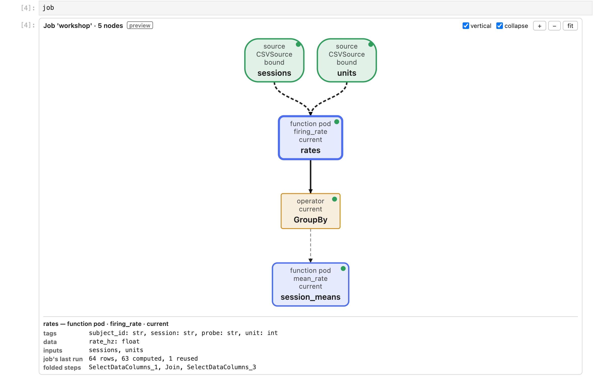
job.diagram() makes the same diagram with options (direction="TB", collapse=True), and
print shows it as text, one node per line with the nodes it reads from. A Pipeline, such
as the job's blueprint job.pipeline, draws itself the same way, without run statuses:
print(job.diagram(collapse=True))# Job 'workshop': 5 nodes# sessions (source · CSVSource · bound)# units (source · CSVSource · bound)# rates (function pod · firing_rate · current) <- sessions, units# GroupBy (operator · current) <- rates# session_means (function pod · mean_rate · current) <- GroupByAn untrusted notebook
Section titled “An untrusted notebook”Where a notebook does not run scripts (an untrusted notebook, a preview on a website), the
picture is still shown, without pan, zoom or selection; open the Nodes table below the
picture for each node's columns and status. JupyterLab runs the scripts of outputs you made
by running a cell. A notebook saved by someone else (or on another machine) opens untrusted:
run its cells again, or trust it (the Trust Notebook command, or
jupyter trust <notebook>.ipynb in a terminal), to get pan, zoom and selection back.
Running asynchronously
Section titled “Running asynchronously”job.run(orchestrator=AsyncPipelineOrchestrator()) is written the same way in a script and in
a notebook. A notebook kernel already runs an event loop. There, job.run(...) runs the job
on a separate thread and waits for it, so the cell blocks until the run ends; the interrupt
button cancels the run. await job.run_async() also works at the top level of a notebook
cell. What the interrupt button does to a function in the middle of a row, and to an
async def function that blocks, is
Running asynchronously, in a script or a notebook.
Classes defined in a notebook cell
Section titled “Classes defined in a notebook cell”A class defined in a notebook is named under __main__, so running its cell again makes a
new class. Define the classes your pods pass around with @op.dataclass: run again, the class
is still the same type, and pods and stored results keep working. An ordinary @dataclass or
a pydantic model run again is a new class, and pods built for the earlier one refuse it. See
op.dataclass in a notebook.
Other notebook front ends
Section titled “Other notebook front ends”The displays are HTML in the cell's output, with the diagram's pan, zoom, selection and
vertical and collapse checkboxes done by a script in that output; the pictures on this page come from
JupyterLab, the front end they are checked in.
- Jupyter Notebook 7 is built on JupyterLab and runs the scripts of trusted outputs as JupyterLab does; it has not been checked separately.
- VS Code and Google Colab show HTML output and run its scripts in their own output frame; the displays have not been checked there.
- Classic Notebook (6) runs the scripts of trusted outputs; it has not been checked.
Where a front end does not run the diagram's script, the diagram shows as in an untrusted notebook.